Classification & non-i.i.d. data

V1.0.1: © Aleksei Tiulpin, PhD, 2025

This notebook shows an end-to-end example on how one can compare two models on a test set where data has block-diagonal covariance (i.e. non-i.i.d. samples measured e.g. from the same patient)

Imports

import stambo
import numpy as np

import matplotlib.pyplot as plt

from sklearn.neighbors import KNeighborsClassifier
from sklearn.linear_model import LogisticRegression
from sklearn.model_selection import StratifiedGroupKFold

SEED = 2025

stambo.__version__

'0.1.5'

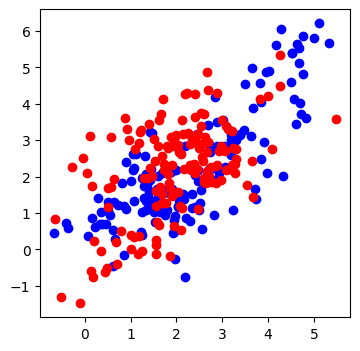
Generating synthetic data with block-diagonal covaraince

We use stambo’s synthetic dataset generation functionality to generate the dataset in question.

np.random.seed(SEED)
n_subjects = 100
n_data = 300

data, y, subject_ids = stambo.synthetic.generate_non_iid_measurements(
    n_data=n_data,
    n_subjects=n_subjects,
    rho=0.8,             # Subject correlation between classes
    subj_sigma=1.0,
    noise_sigma=0.5,
    gamma=0.8,
    mu_cls_1=[2, 2],
    mu_cls_2=[2.1, 2.4],
    overlap=0.2,
    feat_corr=0.5,       # <--- High correlation between Dim 1 and Dim 2
    seed=42
)

plt.figure(figsize=(4, 4))
plt.plot(data[y == 0, 0], data[y == 0, 1], "bo")
plt.plot(data[y == 1, 0], data[y == 1, 1], "ro")
plt.show()

gss = StratifiedGroupKFold(n_splits=3, shuffle=True, random_state=SEED)
train_idx, test_idx = next(gss.split(data, y, groups=subject_ids))

# Split the data into training and testing sets
X_train, X_test = data[train_idx], data[test_idx]
y_train, y_test = y[train_idx], y[test_idx]
groups_train, groups_test = subject_ids[train_idx], subject_ids[test_idx]

# Initialize classifiers
knn = KNeighborsClassifier(n_neighbors=5)
logreg = LogisticRegression()

# Train classifiers
knn.fit(X_train, y_train)
logreg.fit(X_train, y_train)

# Make predictions
knn_predictions = knn.predict(X_test)
logreg_predictions = logreg.predict(X_test)

What we should expect, is that the difference between two models on small data that perform randomly should not be significan. Let’s look at the naive bootstrap:

testing_result = stambo.compare_models(y_test, logreg_predictions, knn_predictions, ("ROCAUC", "AP"),seed=SEED, n_bootstrap=1000)
print(stambo.to_latex(testing_result, m1_name="logreg", m2_name="kNN"))

% \usepackage{booktabs} <-- do not forget to have this imported.
\begin{tabular}{lll} \\
\toprule
\textbf{Model} & \textbf{ROCAUC} & \textbf{AP} \\
\midrule
logreg & $0.45$ [$0.36$-$0.54$] & $0.48$ [$0.39$-$0.58$] \\
kNN & $0.56$ [$0.48$-$0.65$] & $0.54$ [$0.44$-$0.65$] \\
\midrule
Effect size & $0.12$ [$-0.01$-$0.24]$ & $0.06$ [$-0.00$-$0.13]$ \\
\midrule
$p$-value & $0.04$ & $0.05$ \\
\bottomrule
\end{tabular}

We observe statistically significant result here. Let us now correct for clustering:

testing_result = stambo.compare_models(y_test, logreg_predictions, knn_predictions, metrics=("ROCAUC", "AP"), groups=groups_test, seed=SEED, n_bootstrap=1000)
print(stambo.to_latex(testing_result, m1_name="LR", m2_name="kNN"))

% \usepackage{booktabs} <-- do not forget to have this imported.
\begin{tabular}{lll} \\
\toprule
\textbf{Model} & \textbf{ROCAUC} & \textbf{AP} \\
\midrule
LR & $0.45$ [$0.30$-$0.62$] & $0.48$ [$0.24$-$0.74$] \\
kNN & $0.56$ [$0.44$-$0.73$] & $0.54$ [$0.34$-$0.74$] \\
\midrule
Effect size & $0.12$ [$-0.10$-$0.34]$ & $0.06$ [$-0.05$-$0.19]$ \\
\midrule
$p$-value & $0.20$ & $0.18$ \\
\bottomrule
\end{tabular}

Summary: According to conventional bootstrap, we did not find any significant difference between the two models. Once we take into account the subject-level structure, we see that the difference is significant, which is valuable in applications.